Benchmarks

pinnrl-benchmark has two parts: classical baselines, so PINN accuracy has a reference point, and a multi-seed study that compares collocation samplers fairly. Every number below can be reproduced with the commands shown.

Classical baselines

pinnrl-benchmark fdm --pde heat     # explicit finite differences, periodic 1-D heat
pinnrl-benchmark fdm --pde wave     # leap-frog, periodic 1-D travelling wave

Both report the relative L2 error at the final time against the analytical solution, plus the maximum error and the wall time. On the default heat problem (\(\alpha = 0.1\), \(u_0 = \sin 2\pi x\), 101 points), the explicit scheme reaches a relative L2 error of about \(7 \times 10^{-4}\) in about 30 ms. The convergence is second order: doubling the points at a fixed diffusion number cuts the error about four-fold. That's the bar a PINN is measured against on forward problems.

Reference solutions

When there is no closed form, PINNs are scored against high-accuracy numerical references (pinnrl.benchmarks.reference):

Reference	Method	Verification
burgers_reference	Cole–Hopf integral evaluated by a log-sum-exp trapezoid rule	Reproduces Basdevant et al. (1986): \(u_x(0, 1.6037/\pi) = -152.00516\) for \(\nu = 0.01/\pi\); agrees with a fine finite-difference solve to \(7 \times 10^{-5}\)
allen_cahn_reference	Second-order finite differences plus adaptive Runge–Kutta (method of lines) on a grid 8× finer than the output	Grid-converged: doubling the solver grid changes the field by less than \(10^{-5}\) (relative)

Sampling study (experiments B01 and B06)

pinnrl-benchmark sampling --seeds 10 --steps 15000 --checkpoints 50 --workers 4

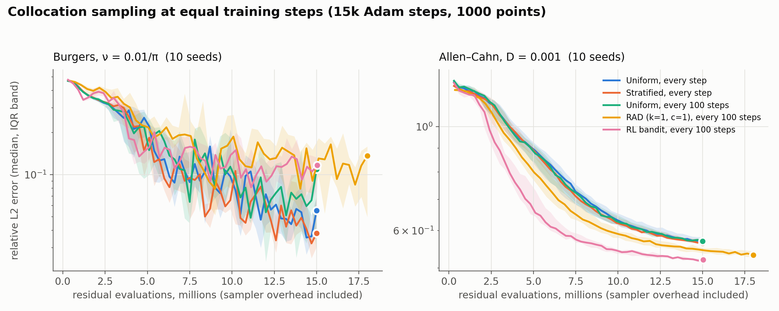
Setup: - The Burgers (\(\nu = 0.01/\pi\)) and Allen–Cahn (\(u_t = 0.001\,u_{xx} + 5(u - u^3)\), \(u_0 = x^2\cos\pi x\)) benchmarks. - A tanh MLP (4 × 64) trained for 15,000 Adam steps on 1,000 points, with 10 paired seeds (identical initial weights across samplers). - Five samplers: - uniform and stratified, with fresh points every step; - uniform refreshed every 100 steps, a control for how often points change; - RAD (k = 1, c = 1) and the RL bandit, also every 100 steps. - Each run records the relative L2 error and the residual evaluations spent, including the sampler's own (RAD +20 %, bandit +0.3 %). Samplers are compared at equal steps (B01) and at equal total evaluations (B06).

PDE	Sampler	Rel. L2, equal steps	vs uniform (paired)	Rel. L2, equal evaluations	vs uniform
Burgers	uniform	0.055	–	0.055	–
	stratified	0.038	6/10, p = 0.63	0.038	6/10, p = 0.63
	RAD	0.136	3/10, p = 0.11	0.090	2/10, p = 0.06
	RL bandit	0.117	1/10, p = 0.06	0.105	2/10, p = 0.01 (worse)
Allen–Cahn	uniform	0.568	–	0.568	–
	RAD	0.533	10/10, p = 0.002	0.547	10/10, p = 0.002
	RL bandit	0.520	10/10, p = 0.002	0.518	10/10, p = 0.002

Errors are medians over 10 seeds; "6/10" counts the seeds on which the sampler beat uniform; p is from a Wilcoxon signed-rank test.

What this says:

• Burgers. No sampler is significantly better than uniform. Seed-to-seed variation (6×) and optimizer noise (the error moves 1.7× between checkpoints at a constant learning rate) swamp any sampling effect. Charged its probe cost, the bandit is significantly worse.
• Allen–Cahn. Adaptive samplers win on every seed and the bandit gets there with about 40 % fewer evaluations early on. But every method stays stuck near the wrong solution (relative error above 0.5).
• Recommendation: use uniform (or stratified) by default. Use residual_based (RAD) when the solution has sharp features, and measure it against uniform at equal budget. Treat --rl as experimental.

The full write-up, with IQRs, the same-cadence control and the follow-ups it motivates (optimizer settling, resampling frequency, Allen–Cahn failure modes), is in experiments/B01_sampling_equal_compute.